SQL Server 2008 : SQLOS schedulers, Wait analysis

1. SQLOS schedulers

SQL Server is a large and complex product with many interconnected components requiring access to common services such as memory allocation and process scheduling. In order to reduce the complexity of each of these components, the SQL Server architecture includes a layer responsible for providing common services.

In SQL Server 2000, this layer, known as the User Mode Scheduler (UMS), was quite thin and had limited responsibilities. Therefore, the ability of the various SQL Server components to take maximum advantage of emerging hardware architecture such as NUMA and hot-add memory was limited. In addressing this, Microsoft rewrote this layer in the SQL Server 2005 release and renamed it the SQL Operating System (SQLOS). Figure 1 illustrates SQLOS in relation to other components.

Figure 1. Shown here are some (but not all) of the SQL Server components. The SQLOS layer provides common services to a number of components.

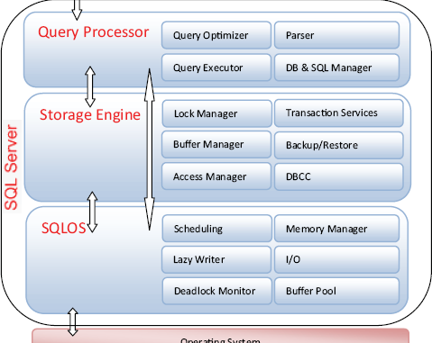
While some of the SQLOS services could be provided by the Windows operating system directly, SQL Server includes them in SQLOS to maximize performance and scalability. Scheduling is a good example of such a service; SQL Server knows its scheduling requirements much better than Windows does. Thus, SQLOS, like the UMS before it, implements scheduling itself.

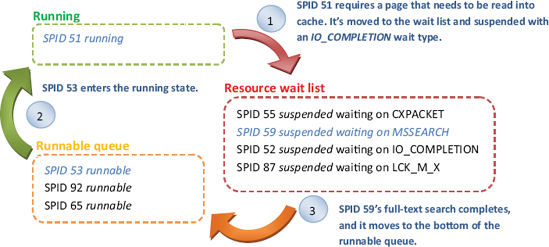
User requests are scheduled for execution by SQLOS using schedulers. SQLOS creates one scheduler for each CPU core that the SQL Server instance has access to. For example, an instance with access to two quad core CPUs would have eight active schedulers. Each of these schedulers executes user requests, or SPIDs, as per the example shown in figure 2.

When a running process requires a resource that isn’t available, for example, a page that’s not found in cache, it’s moved to the wait list until its resource is available, at which point it’s moved to the runnable queue until the CPU becomes available to complete the request. A process moves through the three states until the request is complete, at which point it enters the sleeping state.

From a performance-tuning perspective, what’s very beneficial is the ability to measure the wait list over time, in order to determine which resources are waited on the most. Once this is established, performance tuning becomes a more targeted process by concentrating on the resource bottlenecks. Such a process is commonly called the waits and queues methodology.

Let’s drill down into the various means of analyzing the wait list as part of a performance tuning/troubleshooting process.

2. Wait analysis

Prior to SQL Server 2005, the only means of obtaining information on wait statistics was through the use of the undocumented DBCC SQLPERF(waitstat) command. Fortunately, SQL Server 2005 (and 2008) provides a number of fully documented DMVs for this purpose, making them a central component of wait analysis.

Figure 2. SQLOS uses one scheduler per CPU core. Each scheduler processes SPIDs, which move among the running, suspended, and runnable states/queues.

Let’s look at wait analysis from two perspectives: at a server level using the sys.dm_os_wait_stats DMV and at an individual process level using extended events. This section will focus on measuring waits. In the next section, we’ll look at the association of particular wait types with common performance problems.

2.1. sys.dm_os_wait_stats

As we mentioned earlier, when a session requires a resource that’s not available, it’s moved to the wait list until the resource becomes available. SQLOS aggregates each occurrence of such waits by the wait type and exposes the results through the sys.dm_os_wait_stats DMV. The columns returned by this DMV are as follows:

• wait_type. There are three categories of wait types: resource waits, queue waits, and external waits. Queue waits are used for background tasks such as deadlock monitoring, whereas external waits are used for (among other things) linked server queries and extended stored procedures.

• waiting_tasks_count—This column represents the total number of individual waits recorded for each wait type.

• wait_time_ms—This represents the total amount of time spent waiting on each wait type.

• max_wait_time_ms—This is the maximum amount of time spent for a single occurrence of each wait type.

• signal_wait_time_ms—This represents the time difference between the end of each wait and when the task enters the runnable state, that is, how long tasks spend in the runnable state. This column is important in a performance-tuning exercise because a high signal wait time is indicative of CPU bottlenecks.

As with other DMVs, the results returned by sys.dm_os_wait_stats are applicable only since the last server restart or when the results are manually reset using DBCC SQLPERF (“sys.dm_os_wait_stats”, CLEAR). Further, the results are aggregated across the whole server, that is, the wait statistics for individual statements are not available via this DMV.

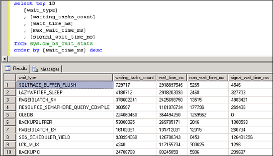
The sys.dm_os_wait_stats DMV makes server-level wait analysis very simple; at any time this DMV can be inspected and ordered as required. For example, figure 3 shows the use of this DMV to return the top 10 wait types in descending order by the total wait time.

Despite the obvious usefulness of this DMV, the one limitation is that it returns all wait types, including system background tasks such as LAZYWRITER_SLEEP, which are not relevant in a performance-analysis/tuning process. Further, we need to manually analyze and rank the returned values in order to determine the most significant waits. In addressing these issues, we can use the track_waitstats and get_waitstats stored procedures.

Figure 3. You can use the output from the sys.dm_os_wait_stats DMV to determine the largest resource waits at a server level.

2.2. Track/get waitstats

The track_waitstats and get_waitstats stored procedures were written by Microsoft’s Tom Davidson for internal use in diagnosing SQL Server performance issues for customer databases. While not officially supported, the code for these stored procedures is publicly available and widely used as part of performance-tuning/troubleshooting exercises.

Originally written to work with DBCC SQLPERF(waitstats), they’ve since been rewritten for the sys.dm_os_wait_stats DMV and renamed to track_waitstats_2005 and get_waitstats_2005. Working with both SQL Server 2005 and 2008, these stored procedures operate as follows:

• The track_waitstats_2005 stored procedure is executed with parameters that specify how many times to sample the sys.dm_os_wait_stats DMV and the interval between each sample. The results are saved to a table called waitstats for later analysis by the get_waitstats_2005 procedure.

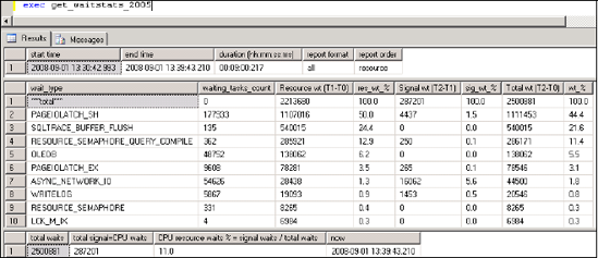
• The get_waitstats_2005 procedure queries the waitstats table and returns aggregated results that exclude irrelevant wait types. Further, as shown in figure 4, the results are broken down by resource waits (wait time minus signal wait time) and signal waits, enabling a quick assessment of CPU pressure.

One of the (many) nice things about these procedures is that they can be called with parameter values that automatically clear the wait statistics, which is helpful in situations in which the monitoring is to be performed while reproducing a known problem. When you clear the waitstats before the event is reproduced, the waits will more accurately represent the waits causing the problem.

Figure 4. The results from get_waitstats_2005 indicate the resources with the highest amount of waits. Irrelevant wait types are excluded.

As mentioned earlier, the wait statistics returned by sys.dm_os_wait_stats are at a server level and represent the cumulative wait statistics from all sessions. While other DMVs, such as sys.dm_os_waiting_tasks, include session-level wait information, the records exist in this DMV only for the period of the wait. Therefore, attempting retrospective wait analysis on a particular session is not possible, unless the information from this DMV is sampled (and saved) on a frequent basis when the session is active. Depending on the length of the session, this may be difficult to do. SQL Server 2008 offers a new alternative in this regard, using the sqlos.wait_info extended event.

2.3. sqlos.wait_info extended event

In SQL Server versions prior to 2008, events such as RPC:Completed can be traced using SQL Server Profiler or a server-side trace. SQL Server 2008 introduces a new event-handling system called extended events, which enables the ability to trace a whole new range of events in addition to those previously available. Extended events enable a complementary troubleshooting technique, which is particularly useful when dealing with difficult-to-diagnose performance problems.

Consider the T-SQL code in listing 1, which creates an extended event of type sqlos.wait_info for SPID 53 and logs its wait type information to file.

Example 1. sqlos.wait_info extended event

-- Create an extended event to log SPID 53's wait info to file
CREATE EVENT SESSION sessionWaits ON SERVER
ADD EVENT sqlos.wait_info
    (WHERE sqlserver.session_id = 53 AND duration > 0)

ADD TARGET package0.asynchronous_file_target
    (SET FILENAME = 'E:\SQL Data\waitStats.xel'

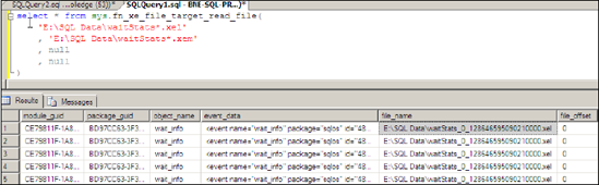
Figure 5. The extended event log file contains XML data (event_data). In our example, the XML would contain information on the wait types for SPID 53.

, METADATAFILE = 'E:\SQL Data\waitStats.xem');
ALTER EVENT SESSION sessionWaits ON SERVER STATE = START

The above code creates an extended event based on waits from SPID 53 with a nonzero duration. Once the event is created, any waits from this SPID will be logged to the specified file. We can read the event log file using the sys.fn_xe_file_target_ read_file function, as shown in figure 5.

The wait type information that we’re interested in is buried within the event_data XML. We can access this more easily using the code shown in listing 2.

Example 2. Viewing wait type information sys.fn_xe_file_target_read_file

-- Retrieve logged Extended Event information from file
CREATE TABLE xeResults (
      event_data XML
)
GO

INSERT INTO xeResults (event_data)
SELECT CAST(event_data as xml) AS event_data
FROM sys.fn_xe_file_target_read_file(
    'E:\SQL Data\waitStats*.xel'
    , 'E:\SQL Data\waitStats*.xem'
    , null
    , null
)
GO

SELECT
    event_data.value('(/event/data/text)[1]','nvarchar(50)') as 'wait_type'
    , event_data.value('(/event/data/value)[3]','int') as 'duration'
    , event_data.value('(/event/data/value)[6]','int') as 'signal_duration'
FROM xeResults
GO

Essentially what we’re doing here is loading the XML into a table and reading the appropriate section to obtain the information we require. The result of this code is shown in figure 6.

Figure 6. We can inspect the event_data column to obtain the wait information produced by the extended event created on sqlos.wait_info.

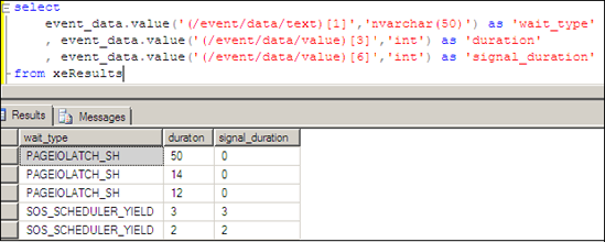
In this particular case, the main wait type for the SPID was PAGEIOLATCH_SH, which we’ll cover shortly. While this is a simple example, it illustrates the ease with which extended events can be created in obtaining a clearer view of system activity, in this case, enabling retrospective wait type analysis on a completed session from a particular SPID.

Let’s turn our attention now to how the information gathered from wait analysis can be combined with Performance Monitor counters and other sources in diagnosing common performance problems.